Tennis Value Betting: How to Calculate Expected Value and Spot Overpriced Odds

html

I spent my first three years betting on tennis chasing winners. My strike rate looked impressive – north of 60% – and I genuinely believed I was beating the market. Then I ran the numbers properly and discovered I was losing money. The problem was not my selections. It was that I had no concept of value. Every profitable bet I have placed in the eight years since comes back to one idea: expected value. If you cannot calculate it, you are guessing, no matter how sophisticated your match analysis looks.

Value betting is the discipline of identifying odds that overstate a player’s chance of losing – or understate their chance of winning. It does not guarantee you win every slip. It guarantees that over hundreds of bets your edge compounds. Football still commands roughly 35% of the global online sports-betting market share, but tennis offers structural advantages for value hunters: two-player contests, granular serve data, and surface transitions that create regular pricing errors. This guide breaks down the expected value formula, shows you how to estimate true probabilities, and maps the mispricing patterns I exploit most often.

The Expected Value Formula Applied to Tennis

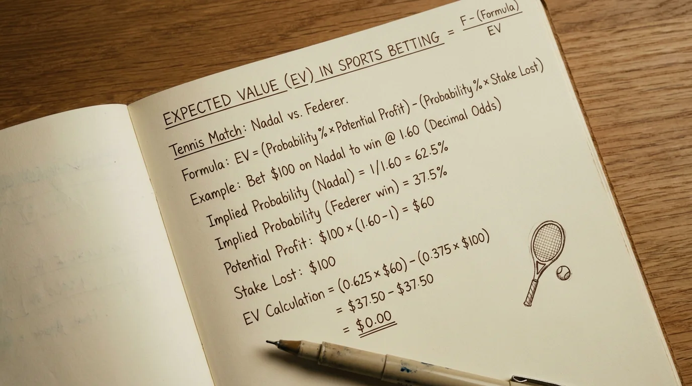
A friend once described expected value to me as “the answer to every bet you will ever place.” Dramatic, perhaps, but not wrong. EV strips away gut feeling and reduces a wager to pure arithmetic – and that is exactly why most recreational bettors avoid it. The formula itself is disarmingly simple:

EV = (Probability of Winning x Net Profit if You Win) – (Probability of Losing x Stake Lost if You Lose)

Suppose you believe a player has a 55% chance of winning a match, and a bookmaker offers decimal odds of 2.10. Your potential net profit on a GBP 10 stake is GBP 11.00 (2.10 x 10 minus the 10 you risked). The EV calculation looks like this: (0.55 x 11) – (0.45 x 10) = 6.05 – 4.50 = +1.55. A positive number means the bet has positive expected value – over time, placing that bet repeatedly should return GBP 1.55 per GBP 10 staked.

Now flip the scenario. If the same player’s true probability is only 45% at the same odds: (0.45 x 11) – (0.55 x 10) = 4.95 – 5.50 = -0.55. Negative EV. You are paying more than the bet is worth. The difference between these two scenarios is not the odds – it is your probability estimate. Get that wrong and nothing else matters.

One thing I learned painfully: EV calculations only become meaningful over volume. A single bet can go either way regardless of its expected value. The edge reveals itself across 200, 500, 1,000 wagers. That is why I log every bet against the EV I estimated at the time of placing it – the gap between predicted EV and actual return tells me whether my probability estimates are calibrated or whether I am fooling myself. If you are consistently overestimating your edge, your “positive EV” bets are nothing of the sort.

When I apply EV to tennis specifically, I focus on match-winner markets first. They are the simplest to model, the most liquid, and the market where my probability estimates have the longest track record. Set betting and over/under games markets can carry bigger EV edges, but the variance is brutal and the probability estimation is far harder to calibrate.

Estimating True Probability: Data, Models and Judgment

Here is where most guides gloss over the hard part. Calculating EV is year-seven maths. Estimating the true probability of a tennis outcome – that is where the actual skill lives. I use a layered approach that blends model output with surface-specific context, and I will walk you through each layer.

The foundation is a ratings-based model. Elo ratings adapted for tennis give you a starting probability for any head-to-head. The system is well-documented: each player carries a numerical rating, and the expected outcome of a match is derived from the difference between ratings. I maintain surface-specific Elo ratings – a player’s hard-court Elo might differ from their clay Elo by 150 points, which translates into a significantly different win probability.

Layer two is serve data. Random-forest models have identified serve strength as the single most powerful predictor of match outcomes, achieving accuracy above 80% in controlled studies. First-serve percentage, first-serve points won, and second-serve points won together explain more variance in match results than ranking, recent form, or head-to-head record. I weight serve data heavily, especially on faster surfaces where the serve advantage amplifies.

Layer three is contextual adjustment. A player returning from a two-month injury layoff will not perform at their Elo rating. A player who has just won a title and is playing a mandatory Masters event three days later might be fatigued or unmotivated. These adjustments are where judgment enters – and where most modellers either over-correct or ignore reality. My rule: never adjust more than 5% from the model output unless you have hard evidence, and log every adjustment so you can review whether your contextual tweaks actually improve accuracy.

Once I have a probability estimate from all three layers, I convert it to implied odds and compare it to the market price. If my estimate says a player wins 58% of the time, the fair decimal odds are 1.72. If the bookmaker offers 1.90, I have a clear positive EV opportunity. If they offer 1.65, I pass – no matter how confident I feel about the player. The statistical foundations behind these models matter more than intuition, and the discipline to trust your numbers over your instinct is what separates profitable bettors from the rest.

Where Tennis Odds Are Most Commonly Mispriced

I keep a spreadsheet of every mispricing pattern I have identified over the past decade. Some dry up as markets get sharper. Others persist because they are driven by structural biases that bookmakers cannot easily correct without alienating recreational customers. Three patterns have been the most durable.

The first is surface transitions. When the tour shifts from clay to grass or grass to hard courts, the market is slow to adjust. Clay-court specialists who have just had strong results carry inflated ratings into the grass season, and their prices remain too short for the first week or two. Conversely, big servers who underperformed on clay suddenly become undervalued on grass. Clay tournaments produce approximately 15% more upsets than grass events, and the transition weeks are precisely when those upset probabilities create the widest pricing gaps. I have found the first two rounds of grass-court tournaments immediately following Roland Garros to be among the most profitable windows of the year.

The second is fatigue and scheduling density. The ATP and WTA calendars are relentless, and back-to-back tournaments create situations where a player is physically compromised but the market still prices them off their peak rating. A player who has just played three consecutive weeks – especially if one included a deep run – faces a measurable drop in serve speed and first-serve percentage. The market accounts for this partially but rarely fully, and the edge is largest in the first round of the subsequent tournament.

The third pattern involves lower-ranked players on their preferred surface. A player ranked 80th in the world who has built their entire game around clay will often be underestimated on that surface against higher-ranked opponents who are more versatile but less surface-specialised. Khalid Ali, CEO of the International Betting Integrity Association, has noted that football and tennis account for the largest share of suspicious betting activity – and it is worth noting that the same lower-tier matches where integrity risks concentrate are also where the most genuine pricing inefficiencies exist. The two are not the same phenomenon, but they share a root cause: bookmakers devote less analytical resource to these markets, which creates opportunity for both sharp bettors and bad actors.

One more pattern worth noting, though it is harder to systematise: retirement risk. When a player carries a known injury into a match, the market adjusts the match-winner odds but rarely prices the retirement scenario correctly into set-betting or over/under markets. If a player retires mid-match, many bookmakers void set bets, which creates asymmetric value opportunities that an EV framework captures neatly.

Turning Theory Into a Repeatable Edge

Knowing the formula is not the edge. Applying it consistently – day after day, tournament after tournament, resisting the temptation to override your model because you “just know” a player will win – that is the edge. I place between 15 and 25 bets per week during the main tour season, and roughly 40% of those are positive EV by my estimates. The rest I pass on.

The practical workflow looks like this: I update my surface-specific Elo ratings after every round of every tournament. Before the next day’s matches, I run each upcoming contest through my model, generate a probability, convert to implied odds, and compare to the best available market price. If my implied odds are at least 5% longer than the market price – meaning I estimate the player has a meaningfully lower chance than the bookmaker does – I stake. If the gap is below 5%, I do not bother, because my probability estimates carry their own error margin.

The staking piece matters enormously too. I use a fractional Kelly approach – roughly a quarter of the Kelly criterion recommendation – because full Kelly is too aggressive for the volatility in tennis markets. A player I rate at 60% to win can still lose five times in a row without any error in my estimate. Quarter-Kelly keeps me in the game during those losing runs.

The final piece is tracking. Every bet goes into a database with the estimated probability, the actual odds, the EV at the time of placement, and the outcome. After every 500 bets, I review my calibration. If I have been estimating 60% probabilities that only win 54% of the time, I adjust. If my grass-court model consistently outperforms my hard-court model, I investigate why. This feedback loop is what makes value betting a system rather than a series of guesses.

Created by the "bettennisonline.com" editorial team.